22  Research sites

Today is going to be a few examples from class Group Projects

22.1 Food Insecurity

The Food sovereignty group has a couple of datasets that need some spatial processing. Here’s a walkthrough of some spatial joins and statistics

22.1.1 Load libraries

── Attaching core tidyverse packages ──────────────────────── tidyverse 2.0.0 ──
✔ dplyr     1.1.2     ✔ readr     2.1.4
✔ forcats   1.0.0     ✔ stringr   1.5.0
✔ ggplot2   3.4.2     ✔ tibble    3.2.1
✔ lubridate 1.9.2     ✔ tidyr     1.3.0
✔ purrr     1.0.1     
── Conflicts ────────────────────────────────────────── tidyverse_conflicts() ──
✖ dplyr::filter() masks stats::filter()
✖ dplyr::lag()    masks stats::lag()
ℹ Use the conflicted package (<http://conflicted.r-lib.org/>) to force all conflicts to become errors
Linking to GEOS 3.9.3, GDAL 3.5.2, PROJ 8.2.1; sf_use_s2() is TRUE

Team Food Sovereignty found a nice resource on Food Insecurity from Feeding America.

Here’s the food insecurity dataset in a google sheet

I can’t read directly from this sheet because I don’t have edit access, so I downloaded it to a spreadsheet. I copied to my own sheet. I tried reading it in via googlesheets4 package but that was causing weird errors, so I downloaded a .csv, moved it to the working directory and imported it that way.

I’ll load the janitor library cause the column names on this worksheet are horrible Excel abominations.

Now read the data with read_csv()

food <- read_csv('MMG2022_2020-2019_FeedingAmerica.xlsx - County.csv')  %>% 
  ##Fix column names
  clean_names() %>% 
  ##select California data for 2020
  filter(state == 'CA') %>% 
  filter(year == 2020)

head(food)
# A tibble: 6 × 23
   fips state county_state    year overall_food_insecur…¹ number_of_food_insec…²
  <dbl> <chr> <chr>          <dbl> <chr>                                   <dbl>
1  6001 CA    Alameda Count…  2020 9.3%                                   154830
2  6003 CA    Alpine County…  2020 11.7%                                     140
3  6005 CA    Amador County…  2020 10.6%                                    4160
4  6007 CA    Butte County,…  2020 14.0%                                   31330
5  6009 CA    Calaveras Cou…  2020 11.4%                                    5240
6  6011 CA    Colusa County…  2020 12.9%                                    2760
# ℹ abbreviated names: ¹​overall_food_insecurity_rate_1_year,
#   ²​number_of_food_insecure_persons_overall_1_year
# ℹ 17 more variables:
#   food_insecurity_rate_among_black_persons_all_ethnicities <chr>,
#   food_insecurity_rate_among_hispanic_persons_any_race <chr>,
#   food_insecurity_rate_among_white_non_hispanic_persons <chr>,
#   low_threshold_in_state <chr>, low_threshold_type <chr>, …

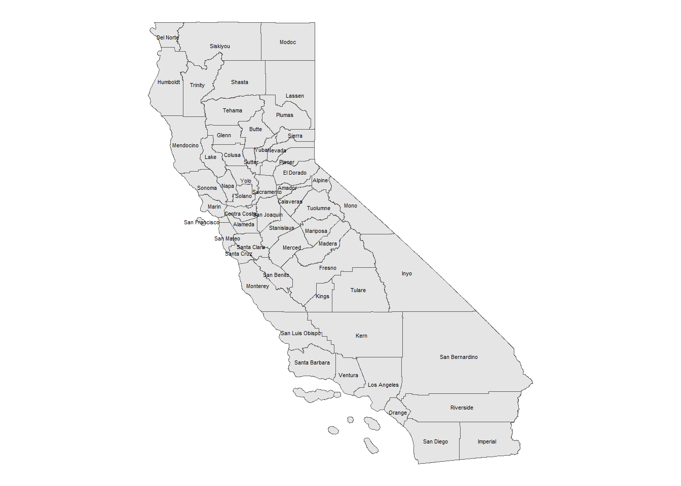
We can add that to a map, if we had a shapefile of California counties. The California open data portal has that info.

Doing this one time, point and click is ok. Here are the steps.

  • Download the zipped shapefile (not code)
  • Move it to your working directory (not code)
  • Unzip/extract the zip file (code or not code - your choice)
  • Read in shapefile using read_sf() - (code)
  • Transform to WGS84 coordinate reference system (code)
  • Make a map (code)
CA_county_dir <- 'CA_counties'

#read the data
CA_county <- read_sf(dsn = CA_county_dir) %>% 
 st_transform("+proj=longlat +ellps=WGS84 +datum=WGS84")

head(CA_county)
Simple feature collection with 6 features and 17 fields
Geometry type: MULTIPOLYGON
Dimension:     XY
Bounding box:  xmin: -121.8626 ymin: 32.75004 xmax: -117.6464 ymax: 39.77688
CRS:           +proj=longlat +ellps=WGS84 +datum=WGS84
# A tibble: 6 × 18
  STATEFP COUNTYFP COUNTYNS GEOID NAME        NAMELSAD LSAD  CLASSFP MTFCC CSAFP
  <chr>   <chr>    <chr>    <chr> <chr>       <chr>    <chr> <chr>   <chr> <chr>
1 06      091      00277310 06091 Sierra      Sierra … 06    H1      G4020 <NA> 
2 06      067      00277298 06067 Sacramento  Sacrame… 06    H1      G4020 472  
3 06      083      00277306 06083 Santa Barb… Santa B… 06    H1      G4020 <NA> 
4 06      009      01675885 06009 Calaveras   Calaver… 06    H1      G4020 <NA> 
5 06      111      00277320 06111 Ventura     Ventura… 06    H1      G4020 348  
6 06      037      00277283 06037 Los Angeles Los Ang… 06    H1      G4020 348  
# ℹ 8 more variables: CBSAFP <chr>, METDIVFP <chr>, FUNCSTAT <chr>,
#   ALAND <dbl>, AWATER <dbl>, INTPTLAT <chr>, INTPTLON <chr>,
#   geometry <MULTIPOLYGON [°]>

Figure 22.1 shows a map of California using ggplot and geom_sf

ggplot(CA_county) +
  geom_sf() +
  theme_void() + 
  geom_sf_text(aes(label = NAME), size = 1.5) +
  labs(x = '', y = '')

Figure 22.1: California Counties

22.1.2 Time for a quick data science lesson

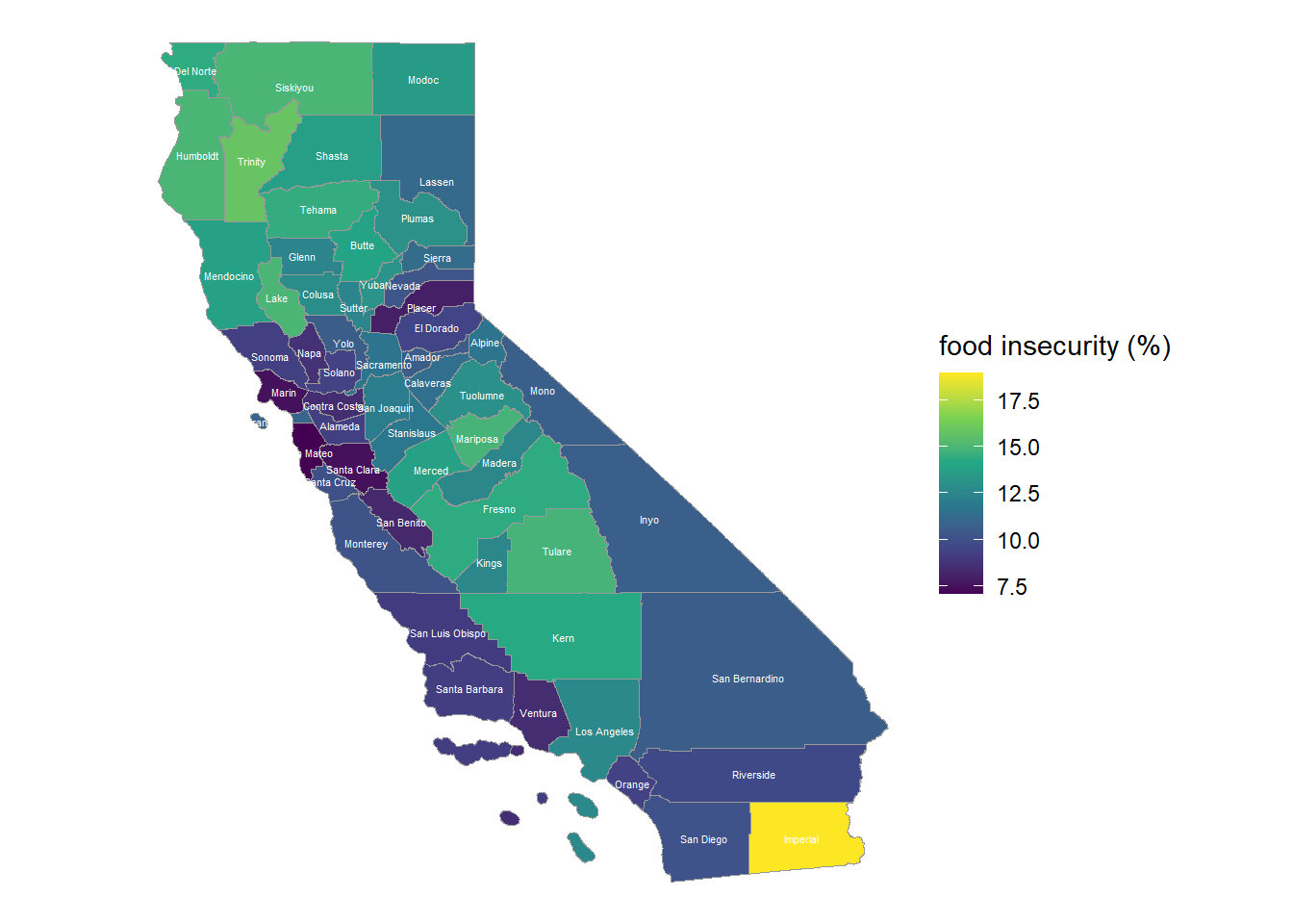
Dataset CA_county has the geospatial information. Dataset food has the food insecurity data but doesn’t have the geospatial information included.

Putting the two datasets together is required to make the map to show spatial patterns in food insecurity. Both datasets have a field that indicates the County Name. The tidyverse dplyr package has functions to join datasets by common variables.

  • inner_join() - keep only records present in both datasets.
  • left_join() - keep all records from the first dataset and only matching variables from the second. Fill missing with NA
  • right_join() - keep all records from the second dataset and only matching variables from the first. Fill missing with NA
  • full_join() - keep all records both datasets - fill NA in any records where dataset is missing from one of the datasets.
  • anti_join() - keep only records in the first dataset that don’t occur in the second dataset.

Join Venn Diagrams - credit Tavareshugo github

For the county case, California has 58 counties, but I will try an inner join to make sure that every county name matches.

Note, the food dataset had an extra bit of text in its county column, we’ll use a tiny bit of language parsing to chop that out so the columns will match exactly.

The string we need to remove is County, California. The function we want is str_remove() from stringr part of the base tidyverse.

food2 <- food %>% 
  mutate(county = str_remove(county_state, ' County, California'))

food2$county
 [1] "Alameda"         "Alpine"          "Amador"          "Butte"          
 [5] "Calaveras"       "Colusa"          "Contra Costa"    "Del Norte"      
 [9] "El Dorado"       "Fresno"          "Glenn"           "Humboldt"       
[13] "Imperial"        "Inyo"            "Kern"            "Kings"          
[17] "Lake"            "Lassen"          "Los Angeles"     "Madera"         
[21] "Marin"           "Mariposa"        "Mendocino"       "Merced"         
[25] "Modoc"           "Mono"            "Monterey"        "Napa"           
[29] "Nevada"          "Orange"          "Placer"          "Plumas"         
[33] "Riverside"       "Sacramento"      "San Benito"      "San Bernardino" 
[37] "San Diego"       "San Francisco"   "San Joaquin"     "San Luis Obispo"
[41] "San Mateo"       "Santa Barbara"   "Santa Clara"     "Santa Cruz"     
[45] "Shasta"          "Sierra"          "Siskiyou"        "Solano"         
[49] "Sonoma"          "Stanislaus"      "Sutter"          "Tehama"         
[53] "Trinity"         "Tulare"          "Tuolumne"        "Ventura"        
[57] "Yolo"            "Yuba"           
food_map <- inner_join(CA_county, food2,
                                by = c('NAME' = 'county')) %>% 
  mutate(pct_food_insecure = as.numeric(str_remove(overall_food_insecurity_rate_1_year, '%')))

head(food_map)
Simple feature collection with 6 features and 41 fields
Geometry type: MULTIPOLYGON
Dimension:     XY
Bounding box:  xmin: -121.8626 ymin: 32.75004 xmax: -117.6464 ymax: 39.77688
CRS:           +proj=longlat +ellps=WGS84 +datum=WGS84
# A tibble: 6 × 42
  STATEFP COUNTYFP COUNTYNS GEOID NAME        NAMELSAD LSAD  CLASSFP MTFCC CSAFP
  <chr>   <chr>    <chr>    <chr> <chr>       <chr>    <chr> <chr>   <chr> <chr>
1 06      091      00277310 06091 Sierra      Sierra … 06    H1      G4020 <NA> 
2 06      067      00277298 06067 Sacramento  Sacrame… 06    H1      G4020 472  
3 06      083      00277306 06083 Santa Barb… Santa B… 06    H1      G4020 <NA> 
4 06      009      01675885 06009 Calaveras   Calaver… 06    H1      G4020 <NA> 
5 06      111      00277320 06111 Ventura     Ventura… 06    H1      G4020 348  
6 06      037      00277283 06037 Los Angeles Los Ang… 06    H1      G4020 348  
# ℹ 32 more variables: CBSAFP <chr>, METDIVFP <chr>, FUNCSTAT <chr>,
#   ALAND <dbl>, AWATER <dbl>, INTPTLAT <chr>, INTPTLON <chr>,
#   geometry <MULTIPOLYGON [°]>, fips <dbl>, state <chr>, county_state <chr>,
#   year <dbl>, overall_food_insecurity_rate_1_year <chr>,
#   number_of_food_insecure_persons_overall_1_year <dbl>,
#   food_insecurity_rate_among_black_persons_all_ethnicities <chr>,
#   food_insecurity_rate_among_hispanic_persons_any_race <chr>, …

Awesome!

Figure 22.2 shows the percent food insecurity by county.

  ggplot(data = food_map, aes(fill = pct_food_insecure)) +
  geom_sf(color = 'grey60') + 
  geom_sf_text(aes(label = NAME), size = 1.5, color = 'white') +
  scale_fill_viridis_c() +
  theme_void() +
  labs(fill = 'food insecurity (%)')
Warning in st_point_on_surface.sfc(sf::st_zm(x)): st_point_on_surface may not
give correct results for longitude/latitude data

Figure 22.2: Percent of food insecure persons by county

22.2 Air Toxics Sacrifice Zones Resources

Toxics Release Inventory Data

National Air Toxics Dashboard

Professor Mike

22.2.1 Toxics Release Inventory

Steps:

  • Download the data from TRI - not code
  • Move it to your working directory (not code)
  • Read in .csv using read_csv() - (code)
  • filter() for pollutants and sites of interest
  • Display on map

22.2.1.1 Import data from working directory

TRI_2021 <- read_csv('2021_us.csv') %>% 
  janitor::clean_names() %>% 
  filter(x34_chemical == 'Ethylene oxide') %>% 
  select(x4_facility_name, x6_city, x12_latitude, x13_longitude, x48_5_1_fugitive_air, x49_5_2_stack_air, x62_on_site_release_total) %>% 
  rename(facility = x4_facility_name,
         city = x6_city,
         lat = x12_latitude,
         lng = x13_longitude,
         emissions = x62_on_site_release_total)
Warning: One or more parsing issues, call `problems()` on your data frame for details,
e.g.:
  dat <- vroom(...)
  problems(dat)
Rows: 76568 Columns: 119
── Column specification ────────────────────────────────────────────────────────
Delimiter: ","
chr (27): 2. TRIFD, 4. FACILITY NAME, 5. STREET ADDRESS, 6. CITY, 7. COUNTY,...
dbl (86): 1. YEAR, 3. FRS ID, 10. BIA, 12. LATITUDE, 13. LONGITUDE, 19. INDU...
lgl  (6): 21. PRIMARY SIC, 22. SIC 2, 23. SIC 3, 24. SIC 4, 25. SIC 5, 26. S...

ℹ Use `spec()` to retrieve the full column specification for this data.
ℹ Specify the column types or set `show_col_types = FALSE` to quiet this message.
head(TRI_2021)
# A tibble: 6 × 7
  facility    city    lat   lng x48_5_1_fugitive_air x49_5_2_stack_air emissions
  <chr>       <chr> <dbl> <dbl>                <dbl>             <dbl>     <dbl>
1 EVONIK CORP RESE…    30   -91                  238              1747      1985
2 EQUISTAR C… PASA…    30   -95                 2321              8302     10623
3 MIDWEST ST… JACK…    37   -90                  211               196       407
4 UNION CARB… SEAD…    29   -97                 1145              3467      4612
5 BECTON DIC… MADI…    34   -83                  959                90      1049
6 TM DEER PA… DEER…    30   -95                    0                 1     10160

Figure 22.3

library(leaflet)
library(htmltools)

leaflet() %>% 
  addTiles() %>% 
  addProviderTiles(provider = providers$Esri.WorldImagery, 
                     group = 'Imagery') %>% 
  addLayersControl(baseGroups = c('Basemap', 'Imagery'), overlayGroups = 'TRI EtO Facilities',
                   options = layersControlOptions(collapsed = FALSE)) %>% 
  addCircles(data = TRI_2021, weight = 1, stroke = FALSE,
             color = 'red',
             radius = ~emissions * 10, popup = ~facility,
             opacity = 0.5,
             group = 'TRI EtO Facilities') %>%
  addCircles(data = TRI_2021, color = 'red', opacity = 0.3)
Assuming "lng" and "lat" are longitude and latitude, respectively

Figure 22.3: Ethylene oxide facilities reporting to TRI in 2021

Examine this map and tell me at least three things that are wrong with it.