Environmental Data Visualization - 16 Data Science 101

16.1.1 `st_transform()`

st_transform() transforms or converts coordinates of simple feature geospatial data. Spatial projections are fraught with peril in geospatial visualizations. Our first function is one that has been used a bunch of times - st_transform(). Leaflet needs its data transformed into WGS84 and st_transform() is the function that makes the coordinate reference system go the right place.

URL.path <- 'https://raw.githubusercontent.com/RadicalResearchLLC/EDVcourse/main/CalEJ4/CalEJ.geoJSON'
SoCalEJ <- st_read(URL.path) %>% 
  st_transform("+proj=longlat +ellps=WGS84 +datum=WGS84")

Reading layer `CalEJ' from data source 
  `https://raw.githubusercontent.com/RadicalResearchLLC/EDVcourse/main/CalEJ4/CalEJ.geoJSON' 
  using driver `GeoJSON'
Simple feature collection with 3747 features and 66 fields
Geometry type: MULTIPOLYGON
Dimension:     XY
Bounding box:  xmin: 97418.38 ymin: -577885.1 xmax: 539719.6 ymax: -236300
Projected CRS: NAD83 / California Albers

WH.url <- 'https://raw.githubusercontent.com/RadicalResearchLLC/WarehouseMap/main/WarehouseCITY/geoJSON/finalParcels.geojson'
warehouses <- st_read(WH.url) %>% 
  st_transform("+proj=longlat +ellps=WGS84 +datum=WGS84")

Reading layer `finalParcels' from data source 
  `https://raw.githubusercontent.com/RadicalResearchLLC/WarehouseMap/main/WarehouseCITY/geoJSON/finalParcels.geojson' 
  using driver `GeoJSON'
Simple feature collection with 8606 features and 11 fields
Geometry type: POLYGON
Dimension:     XY
Bounding box:  xmin: -118.8037 ymin: 33.43325 xmax: -114.4085 ymax: 35.55527
Geodetic CRS:  WGS 84

16.1.2 `janitor::clean_names()`

The first step in being able to deal with a dataset is to have the names of the variables comport with standard R naming format. clean_names() gets rid of those spaces and standardizes the capitalization of letters for column names.

If your dataset column names have spaces or strange characters (parentheses, $, or /), the best way to deal with that is to instantly run clean_names(). R functions do not like special characters in variable names.

In Chapter 12 we used janitor::clean_names() to fix the import of the ecological footprint excel spreadsheet. Here’s the example again.

16.1.3 FIXME - add a section on ‘clean_names()’ using SoCalEJ

16.1.4 `filter()`

filter() is used to subset a data table, retaining any rows that meet the conditions of the filter.

filter() is used on numbers by applying operators (e.g., >, =, <, >=, <=).
filter() can be applied on character strings by using the identity operator ==.
filter() can be applied to multiple character strings by using the %in% operator on lists.

In the first example, filter()was applied to remove the values that were set at -999; we only believed values from 0-100 were reasonable. Figure 16.1 uses filter() to remove those values. I’ve also shown an example without the filter applied in Figure 16.2 . Not removing those rows messes up our visualization.

SoCalEJ %>% 
  filter(AsthmaP >= 0) %>% 
  ggplot(aes(x = County, y = AsthmaP)) +
  geom_boxplot()

Figure 16.1: Asthma census tract distribution by county

SoCalEJ %>% 
  #filter()
  ggplot(aes(x = County, y = AsthmaP)) +
  geom_boxplot()

Figure 16.2: Asthma census tract distribution by county without filter

In Chapter 11 we also applied filter in two successive data transformations that are good examples of data munging. After creating a narrow data set, we apply filter(value >=0) to remove all negative values. Then we applied filter(variable %in% c('OzoneP', 'DieselPM_P', 'PolBurdP')) to select three specific variable choices out of the 55 we had available. If we exclude that second filter, the plot becomes crazy busy.

# select socioeconomic indicators and make them narrow - only include counties above 70%
SoCal_narrow <- SoCalEJ %>% 
  st_set_geometry(value = NULL) %>% 
  pivot_longer(cols = c(5:66), names_to = 'variable', values_to = 'value') %>% 
  filter(value >=0)

SoCal_narrow %>% 
  filter(variable %in% c('OzoneP', 'DieselPM_P', 'PolBurdP')) %>% 
  ggplot(aes(x = County, y = value, fill= variable)) +
  geom_boxplot()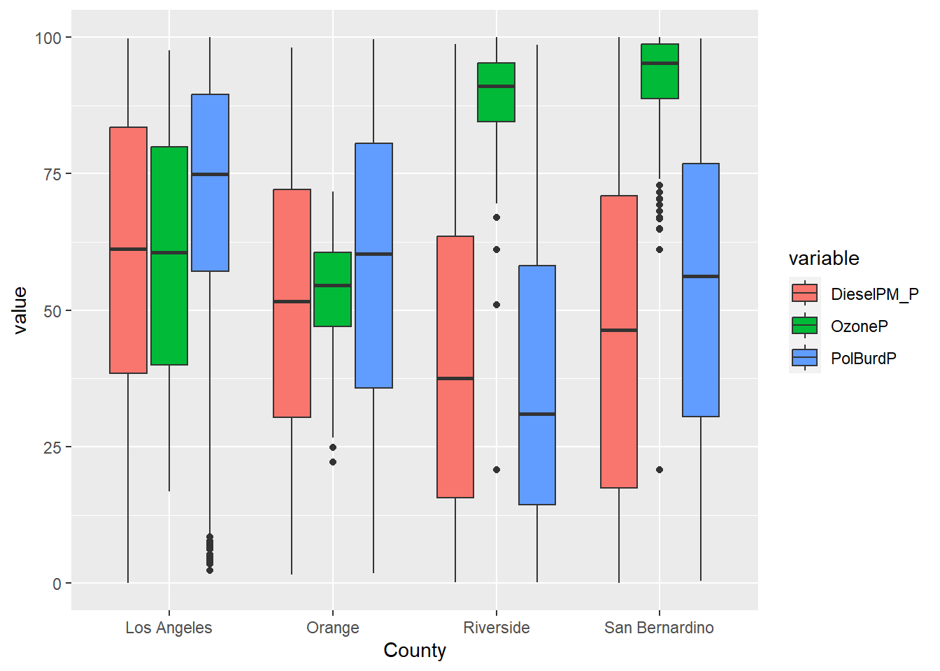

SoCal_narrow %>% 
  #filter(variable %in% c('OzoneP', 'DieselPM_P', 'PolBurdP')) %>% 
  ggplot(aes(x = County, y = value, fill= variable)) +
  geom_boxplot()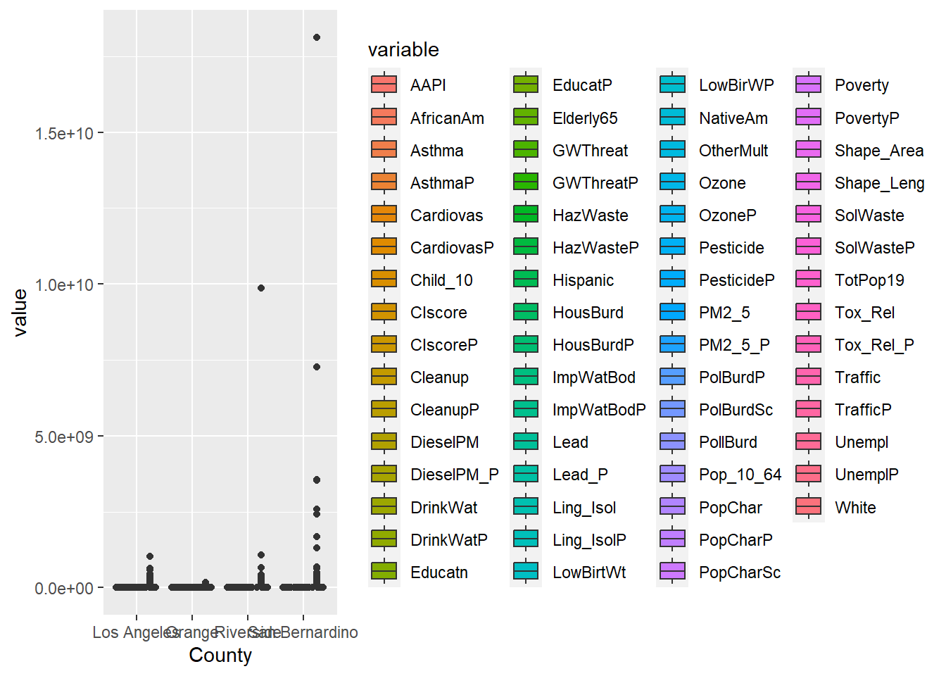

16.1.5 `select()`

select() variables (i.e., columns) in a data table for retention.

select() can be applied to subsets column number or name.
select() also has some pattern matching helpers.

?sec-EJTheory included an example of using select() on the SoCalEJ dataset. The raw dataset is MESSY!

## This is a test import of the first 25 rows of an 18,000 row dataset
TRI_2021_raw <- read_csv('2021_us.csv', n_max = 25) #%>% 
head(TRI_2021_raw)

# A tibble: 6 × 119
  `1. YEAR` `2. TRIFD`       `3. FRS ID` `4. FACILITY NAME`  `5. STREET ADDRESS`
      <dbl> <chr>                  <dbl> <chr>               <chr>              
1      2021 65301SRRBL1400W 110000444421 SIERRA BULLETS L.L… 1400 W HENRY ST    
2      2021 46506MLLRB225IN 110000398542 RBC PRECISION PROD… 225 INDUSTRIAL DR  
3      2021 3211WBRDDC4FENT 110057678197 BRADDOCK METALLURG… 400 FENTRESS BLVD  
4      2021 76712CCCLF8400I 110000460563 COCA-COLA NORTH AM… 8400 IMPERIAL DR   
5      2021 3355WMTTLR1571N 110070941744 METTLER TOLEDO      1571 NORTHPOINTE P…
6      2021 3355WMTTLR1571N 110070941744 METTLER TOLEDO      1571 NORTHPOINTE P…
# ℹ 114 more variables: `6. CITY` <chr>, `7. COUNTY` <chr>, `8. ST` <chr>,
#   `9. ZIP` <chr>, `10. BIA` <lgl>, `11. TRIBE` <lgl>, `12. LATITUDE` <dbl>,
#   `13. LONGITUDE` <dbl>, `14. HORIZONTAL DATUM` <chr>,
#   `15. PARENT CO NAME` <chr>, `16. PARENT CO DB NUM` <chr>,
#   `17. STANDARD PARENT CO NAME` <chr>, `18. FEDERAL FACILITY` <chr>,
#   `19. INDUSTRY SECTOR CODE` <dbl>, `20. INDUSTRY SECTOR` <chr>,
#   `21. PRIMARY SIC` <lgl>, `22. SIC 2` <lgl>, `23. SIC 3` <lgl>, …

## This dataset is MESSY! Time to munge!

TRI_2021 <- read_csv('2021_us.csv') %>% 
  # make variable names better
  janitor::clean_names() %>% 
  # keep only Ethylene oxide facilities
  filter(x34_chemical == 'Ethylene oxide') %>% 
  # keep only the name, city, lat/lng, and emissions total columns
  select(x4_facility_name, x6_city, x12_latitude, x13_longitude,    x62_on_site_release_total) %>% 
  rename(facility = x4_facility_name,
         city = x6_city,
         lat = x12_latitude,
         lng = x13_longitude,
         emissions = x62_on_site_release_total)

head(TRI_2021)

# A tibble: 6 × 5
  facility                                   city        lat   lng emissions
  <chr>                                      <chr>     <dbl> <dbl>     <dbl>
1 EVONIK CORP                                RESERVE      30   -91      1985
2 EQUISTAR CHEMICALS BAYPORT CHEMICALS PLANT PASADENA     30   -95     10623
3 MIDWEST STERILIZATION CORP                 JACKSON      37   -90       407
4 UNION CARBIDE CORP SEADRIFT PLANT          SEADRIFT     29   -97      4612
5 BECTON DICKINSON & CO MADISON OPERATIONS   MADISON      34   -83      1049
6 TM DEER PARK SERVICES LP                   DEER PARK    30   -95     10160

Figure 22.3

library(leaflet)
library(htmltools)

leaflet() %>% 
  addTiles() %>% 
  addProviderTiles(provider = providers$Esri.WorldImagery, 
                     group = 'Imagery') %>% 
  addLayersControl(baseGroups = c('Basemap', 'Imagery'), overlayGroups = 'TRI EtO Facilities',
                   options = layersControlOptions(collapsed = FALSE)) %>% 
  addCircles(data = TRI_2021, color = 'red', opacity = 0.3) %>% 
  addCircles(data = TRI_2021, weight = 1, stroke = FALSE,
             color = 'red',
             radius = ~emissions * 10, popup = ~facility,
             opacity = 0.5,
             group = 'TRI EtO Facilities')

Figure 16.3: Ethylene oxide facilities reporting to TRI in 2021

16.1.6 `mutate()`

mutate() adds new variables and preserves existing ones. mutate() can be used to overwrite existing variables - careful with name choices.

This is a great function for synthesizing information, transformations, and combining variables.

changing units - use mutate()
creating a rate or normalizing data - use mutate()
need a new variable or category - use mutate()

I used mutate() to create a decimal date function for our CH₄ visualizations in ?sec-import. I used mutate() to correct the spelling of San Bernardino in Chapter 9, in combination with the ifelse() function. I used mutate() in Chapter 22 to calculate volumes of rain by multiplying precipitation values (inches) by area (m²) of counties.

Let’s use mutate() to convert the TRI ethylene oxide emissions from pounds to kilograms to avoid imperialism.

1 pound = 0.453592 kilograms

TRI_2021 <- TRI_2021 %>% 
  mutate(emissions_kg = emissions*0.453592)
head(TRI_2021)

# A tibble: 6 × 6
  facility                              city    lat   lng emissions emissions_kg
  <chr>                                 <chr> <dbl> <dbl>     <dbl>        <dbl>
1 EVONIK CORP                           RESE…    30   -91      1985         900.
2 EQUISTAR CHEMICALS BAYPORT CHEMICALS… PASA…    30   -95     10623        4819.
3 MIDWEST STERILIZATION CORP            JACK…    37   -90       407         185.
4 UNION CARBIDE CORP SEADRIFT PLANT     SEAD…    29   -97      4612        2092.
5 BECTON DICKINSON & CO MADISON OPERAT… MADI…    34   -83      1049         476.
6 TM DEER PARK SERVICES LP              DEER…    30   -95     10160        4608.

16.1.7 `summarize()`

summarize() creates a new table that reduces a dataset to a summary of all observations. When combined with the group_by() function, it allows extremely powerful manipulation and generation of summary statistics about a dataset.

I have not demonstrated summarize() yet in this class, which is a major deficiency on my part. Let’s examine it with TRI_2021.

EtO_summary <- TRI_2021 %>% 
  summarize(count = n(), sum = sum(emissions), average = mean(emissions),
            max = max(emissions), min = min(emissions), 
            stdev = sd(emissions))

library(kableExtra)
# This is just a fancy table instead of showing the normal output
kable(EtO_summary)

count	sum	average	max	min	stdev
118	167320	1417.966	18980	0	3011.106

A more interesting example includes the group_by() function. This function identifies categories to summarize the data by. The SoCalEJ_narrow dataset has some simple grouping categories that can be used to show this.

SoCal_basic <- SoCal_narrow %>% 
  group_by(variable) %>% 
  summarize(count = n(), average = mean(value), min = min(value), max =       max(value), stdev = sd(value))

kable(SoCal_basic, digits = 1, caption = 'An example summary Table',
      format.args = list(scientific = FALSE))

An example summary Table
variable	count	average	min	max	stdev
AAPI	3728	13.3	0.0	87.6	14.8
AfricanAm	3728	6.4	0.0	84.7	10.1
Asthma	3737	50.4	4.3	202.6	26.9
AsthmaP	3737	49.7	0.0	99.9	27.7
CIscore	3693	33.9	1.8	82.4	16.7
CIscoreP	3693	59.9	0.2	100.0	27.3
Cardiovas	3737	14.3	3.9	40.9	5.2
CardiovasP	3737	55.4	0.0	100.0	27.6
Child_10	3728	12.0	0.0	51.5	4.3
Cleanup	3747	9.8	0.0	276.2	16.5
CleanupP	3747	37.6	0.0	100.0	34.1
DieselPM	3747	0.3	0.0	14.6	0.3
DieselPM_P	3747	54.7	0.0	100.0	27.8
DrinkWat	3727	565.3	33.9	1161.1	195.8
DrinkWatP	3727	62.8	0.1	100.0	25.3
EducatP	3688	55.7	0.0	100.0	29.1
Educatn	3688	20.4	0.0	72.9	15.4
Elderly65	3728	14.1	0.0	100.0	8.3
GWThreat	3747	11.5	0.0	348.4	22.0
GWThreatP	3747	31.6	0.0	99.9	31.1
HazWaste	3747	0.7	0.0	22.3	1.6
HazWasteP	3747	49.5	0.0	100.0	29.8
Hispanic	3728	46.1	0.0	100.0	27.4
HousBurd	3673	20.7	1.6	78.2	8.6
HousBurdP	3673	58.2	0.0	100.0	28.2
ImpWatBod	3747	2.7	0.0	29.0	4.1
ImpWatBodP	3747	23.8	0.0	99.7	31.0
Lead	3695	54.2	0.0	99.4	24.0
Lead_P	3695	56.4	0.0	100.0	29.8
Ling_Isol	3607	11.7	0.0	100.0	10.3
Ling_IsolP	3607	54.9	0.0	100.0	29.1
LowBirWP	3642	53.2	0.0	100.0	28.5
LowBirtWt	3642	5.2	0.0	12.7	1.6
NativeAm	3728	0.3	0.0	100.0	2.5
OtherMult	3728	2.6	0.0	14.8	2.3
Ozone	3747	0.1	0.0	0.1	0.0
OzoneP	3747	65.3	16.8	100.0	23.7
PM2_5	3747	11.3	4.8	15.4	1.5
PM2_5_P	3747	66.8	0.9	99.4	21.9
Pesticide	3747	18.2	0.0	16311.6	353.9
PesticideP	3747	9.4	0.0	99.1	20.1
PolBurdP	3747	63.1	0.2	100.0	26.8
PolBurdSc	3747	5.9	1.6	10.0	1.5
PollBurd	3747	48.4	12.9	81.9	12.1
PopChar	3693	53.9	4.4	95.0	20.0
PopCharP	3693	55.7	0.1	99.9	28.2
PopCharSc	3693	5.6	0.5	9.9	2.1
Pop_10_64	3728	73.9	0.0	100.0	7.2
Poverty	3703	33.7	2.1	93.2	18.1
PovertyP	3703	54.2	0.1	100.0	28.1
Shape_Area	3747	22329204.5	70452.5	18117312341.2	379230046.0
Shape_Leng	3747	9778.8	1159.5	807614.6	24691.9
SolWaste	3747	2.1	0.0	64.2	4.0
SolWasteP	3747	29.9	0.0	100.0	32.2
TotPop19	3747	4753.2	0.0	23390.0	2127.5
Tox_Rel	3747	3018.0	0.0	96985.6	4902.5
Tox_Rel_P	3747	69.5	0.0	100.0	24.3
Traffic	3728	1340.7	20.7	6836.5	954.4
TrafficP	3728	58.3	0.0	100.0	27.2
Unempl	3607	6.3	0.0	43.9	3.5
UnemplP	3607	52.3	0.0	100.0	27.3
White	3728	31.2	0.0	97.4	25.0

And of course, we can combine our functions to dig even deeper. This example focuses on just a few variables to group the data into smaller subsets of County.

SoCal_complicated <- SoCal_narrow %>% 
  filter(variable %in% c('CIscoreP', 'AsthmaP', 'LowBirWP', 'CardiovasP')) %>% 
  group_by(variable, County) %>% 
  summarize(count = n(), average = mean(value), min = min(value), max =       max(value), stdev = sd(value))

`summarise()` has grouped output by 'variable'. You can override using the
`.groups` argument.

kable(SoCal_complicated, digits = 1, caption = 'An example summary Table',
      format.args = list(scientific = FALSE))

An example summary Table
variable	County	count	average	min	max	stdev
AsthmaP	Los Angeles	2334	53.4	0.0	99.3	28.2
AsthmaP	Orange	582	27.9	0.1	70.4	18.4
AsthmaP	Riverside	453	49.6	2.9	94.1	22.5
AsthmaP	San Bernardino	368	60.9	0.9	99.9	24.5
CIscoreP	Los Angeles	2297	66.2	0.3	100.0	26.2
CIscoreP	Orange	580	42.4	0.2	97.4	26.1
CIscoreP	Riverside	450	48.8	1.1	99.3	23.9
CIscoreP	San Bernardino	366	61.2	4.3	99.6	23.0
CardiovasP	Los Angeles	2334	54.4	0.0	99.2	27.0
CardiovasP	Orange	582	33.0	0.2	77.4	17.7
CardiovasP	Riverside	453	71.9	2.6	99.4	22.5
CardiovasP	San Bernardino	368	77.3	14.2	100.0	19.0
LowBirWP	Los Angeles	2279	55.4	0.0	99.9	29.2
LowBirWP	Orange	571	42.8	0.0	99.4	26.5
LowBirWP	Riverside	430	49.7	0.1	100.0	25.8
LowBirWP	San Bernardino	362	60.1	0.2	99.8	25.6

16.1 Introduction

16.1.1 st_transform()

16.1.2 janitor::clean_names()

16.1.3 FIXME - add a section on ‘clean_names()’ using SoCalEJ

16.1.4 filter()

16.1.5 select()

16.1.6 mutate()

16.1.7 summarize()

16.1.1 `st_transform()`

16.1.2 `janitor::clean_names()`

16.1.4 `filter()`

16.1.5 `select()`

16.1.6 `mutate()`

16.1.7 `summarize()`