27  heatmap

Let’s make a heatmap or two

27.1 Libraries

The usual suspects.

library(sf)
library(tidyverse)
library(leaflet)

27.2 New Packages for today

leaflet.extras - this has an addHeatmap() function for leaflet maps. rmapshaper - this has ms_simplify() to reduce the complexity of polygons and make them faster to render.

install.packages(c('rmapshaper', 'leaflet.extras'))

library(rmapshaper)
library(leaflet.extras)

27.3 Import Data

Check Drop Box for a water hyacinth observation dataset from CalFlora named Eich_Data.csv provided by Team Invasives.

Water Hyacinth - wikimedia

waterHyacinth <- read_csv('Eich_Data.csv') %>% 
  select(SciName, ObsDate, Latitude, Longitude)

New names:
• `` -> `...1`

Warning: One or more parsing issues, call `problems()` on your data frame for details,
e.g.:
  dat <- vroom(...)
  problems(dat)

Rows: 12676 Columns: 7
── Column specification ────────────────────────────────────────────────────────
Delimiter: ","
chr (3): SciName, ObsDate, geometry
dbl (4): ...1, ID, Latitude, Longitude

ℹ Use `spec()` to retrieve the full column specification for this data.
ℹ Specify the column types or set `show_col_types = FALSE` to quiet this message.

27.4 Make a simple Heatmap in Leaflet

Instead of adding the 12,000+ markers directly, we will show the density of observations using a heatmap. The addHeatmap() in leaflet.extras is a pretty straightforward function. The key arguments are radius and blur. I’ll show a map with some reasonable values for this dataset.

Figure 27.1 shows the heatmap.

leaflet() %>% 
  addTiles() %>% 
  addHeatmap(data = waterHyacinth,
             radius = 10,
             blur = 15)

Assuming "Longitude" and "Latitude" are longitude and latitude, respectively

Figure 27.1: Heatmap of water hyacinth observations in California.

27.4.1 Exercise 1

• Change the value of radius argument and see how the heatmap changes.
• Change the value of blur argument and see how the heatmap changes
• Add a setView() to the map and see how the heatmap changes at a non-default zoom setting.

27.5 Heatmaps 2 - ggplot methods for looking at small multiples.

27.5.1 Import California Counties data

Import the county dataset from lesson 22.1.1.

CA_county <- read_sf(dsn = 'CA_counties') %>% 
 st_transform(crs = 4326)

27.5.2 Make a heatmap in ggplot

The function stat_density2d() is used to make a heatmap in ggplot.

Figure 27.2 shows how that’s done.

ggplot() +
  geom_sf(data = CA_county, fill = 'white') +
  geom_density_2d_filled(data = waterHyacinth,
                  aes(x= Longitude,
                      y= Latitude),
             alpha = 0.8,
             breaks = c(0.0001, 0.001, 0.01, 0.1, 1, 10, 100)) +
  theme_void() +
  labs(fill = 'Water hyacinth density')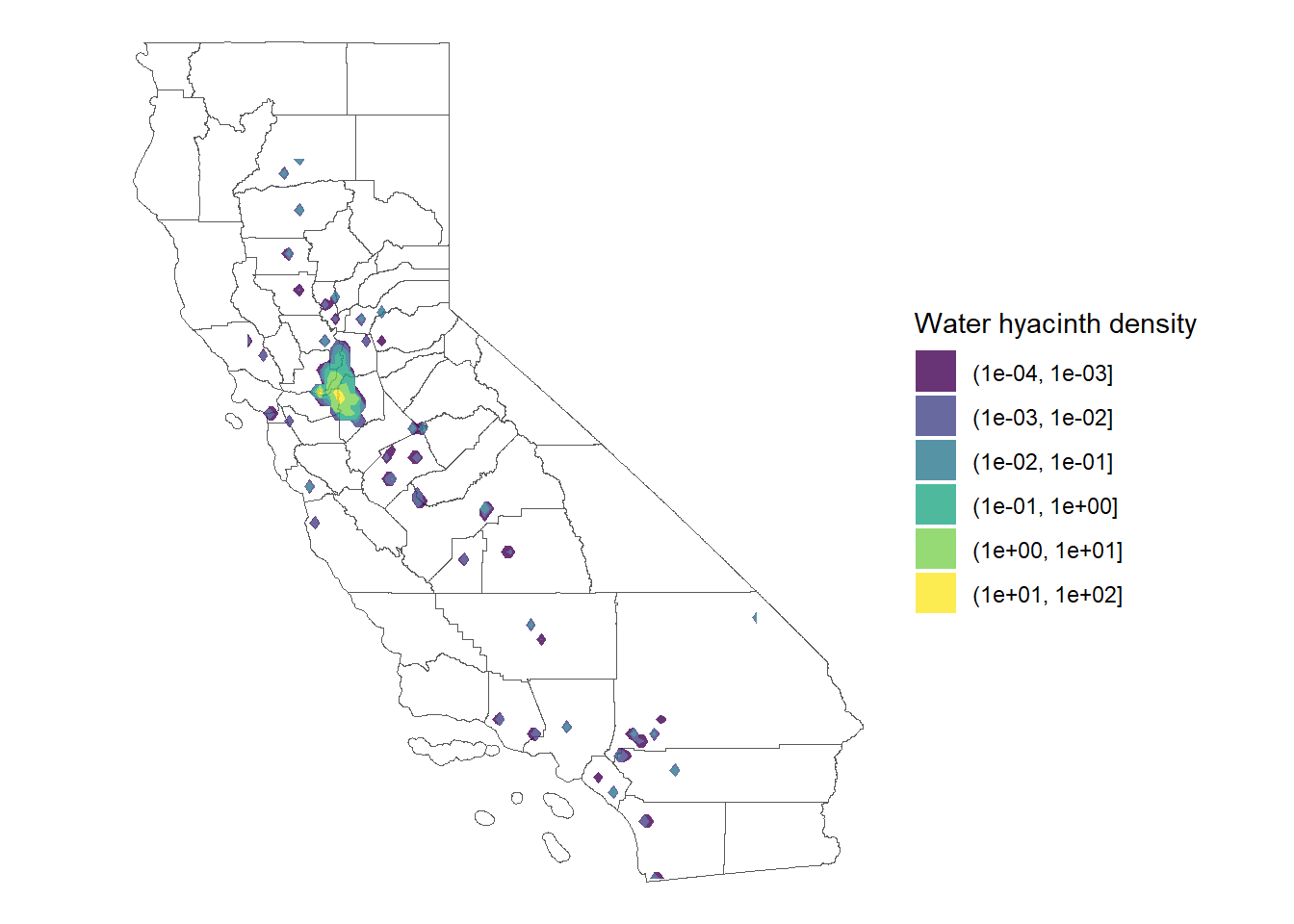

Figure 27.2: Water hyacinth heatmap in ggplot

There’s a couple of wonky things about this map. Defaults for the levels are pretty weird, so I had to add the breaks to show the density of observations in a more reasonable way.

27.5.3 Exercise 2

• Try out stat_density_2d(), geom_density_2d(), and/or stat_density_2d_filled() for variations.
• Try different break levels and see how the map changes.

27.6 Facet_wrap with densities

As always, combining methods makes this more usefu.

The waterHyacinth data has some observations with dates. I wanted to do see how these change over time, but only 43 out of the 12000+ observations had reasonable years, so we’re going to skip that as something that can be done with this dataset.

27.7 Simplifying polygons

One last example trick. Another dataset Team invasives was working on was extreme in its polygons.

Here is a bit of code to tone that down and simplify the polygons for faster rendering maps.

The data is from California Freshwater Species Database.
The rmapshaper package has a function called ms_simplify() which helps to make a simpler map for display.

species <- sf::st_read(dsn = 'ds1197/ds1197.gdb',
                       quiet = TRUE) %>% 
  st_transform(crs = 4326)

Warning in evalq((function (..., call. = TRUE, immediate. = FALSE, noBreaks. =
FALSE, : automatically selected the first layer in a data source containing more
than one.

Warning in CPL_read_ogr(dsn, layer, query, as.character(options), quiet, :
GDAL Message 1: organizePolygons() received a polygon with more than 100 parts.
The processing may be really slow. You can skip the processing by setting
METHOD=SKIP.

species2 <- ms_simplify(species)

object.size(species)

93290552 bytes

object.size(species2)

8994872 bytes

Figure 27.3 shows the simplified map.

palSpecies <- colorNumeric(palette = 'OrRd',
                            domain = species2$Vulnerable_Species_Count)

leaflet() %>% 
  addTiles() %>% 
  addPolygons(data = species2,
              weight = 0.1,
              color =   ~palSpecies(Vulnerable_Species_Count),
              fillOpacity = 0.6) %>% 
  addLegend(data = species2,
            title= 'Vulnerable Freshwater Species',
            pal = palSpecies,
            values = ~Vulnerable_Species_Count)

Figure 27.3: Vulnerable species counts