26 KQED
Today I show an example of a map I made yesterday for NPR’s KQED station in the Bay Area.
26.1 KQED NPR radio
My neighbor Jen and Professor Phillips were on KQED’s California Report talking about warehouses.
26.2 Libraries
26.3 Datasets
26.3.1 Warehouses
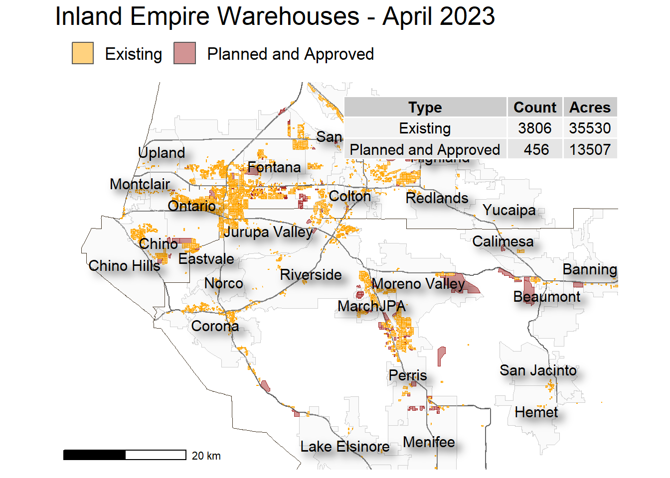
WH.url <- 'https://raw.githubusercontent.com/RadicalResearchLLC/WarehouseMap/main/WarehouseCITY/geoJSON/finalParcels.geojson'
warehouses <- st_read(WH.url, quiet = TRUE) %>%
  filter(county %in% c('Riverside','San Bernardino')) %>%
  st_transform("+proj=longlat +ellps=WGS84 +datum=WGS84") %>%
  select(geometry) %>%
  mutate(type = 'Existing')

plannedWH.url <- 'https://raw.githubusercontent.com/RadicalResearchLLC/PlannedWarehouses/main/plannedWarehouses.geojson'
plannedWH <- st_read(plannedWH.url, quiet = TRUE) %>%
  st_transform("+proj=longlat +ellps=WGS84 +datum=WGS84") %>%
  select(geometry) %>%
  mutate(type = 'Planned and Approved')

wh <- bind_rows(plannedWH, warehouses)
area <- st_area(wh)

stats <- wh %>%
  st_set_geometry(value = NULL) %>%
  mutate(shape = as.numeric(area*10.7639)) %>%
  group_by(type) %>%
  summarize(Count = n(), areaSqFt = sum(shape)) %>%
  mutate(Acres = round(areaSqFt/43560,0)) %>%
  rename(Type = type) %>%
  select(Type, Count, Acres)
26.3.2 Jurisdictional Boundaries
Load cities and county boundaries.
City boundaries are from SCAG.
County boundaries are from California open data, same as we pulled in Lecture 22
jurisdictions <- st_read(dsn = 'C:/Dev/IE_TopWarehouseCities/jurisdictions.geojson', quiet = TRUE) %>%
  filter(lsad == 25 | name == 'MarchJPA') %>%
  st_transform("+proj=longlat +ellps=WGS84 +datum=WGS84")

areaValue2 <- st_area(jurisdictions)

counties <- sf::st_read(dsn = 'C:/Dev/CA_spatial_data/CA_counties', quiet = TRUE) %>%
  filter(NAME %in% c('Riverside', 'San Bernardino')) %>%
  select(geometry) %>%
  st_transform(crs = 4326)
26.3.3 Freeways
Californians love roads. Freeways in particular.
Here is a freeways dataset
This dataset is strange in that it has Z-axis data (i.e., elevation). Leaflet doesn’t like Z or M axis data so one needs to fix the geometry to get rid of that.
st_zm() is a function to fix the polyline geometry to be 2-dimensional.
26.3.4 Munging
I want to only include cities in the IE valleys and avoid the high (Mojave) and low (Colorado) deserts.
26.4 Make a nice map
First, let’s install a couple of new packages used for some neato effects.
#multipackage install
install.packages(c('ggpmisc', 'ggfx', 'ggspatial'))library(ggpmisc)
library(ggthemes)
library(ggfx)
library(ggspatial)
IE_WH_map <- ggplot() +
geom_sf(data = highway2, color = 'gray40', size = 1) +
geom_sf(data = juris2, alpha = 0.2, fill = 'gray90',
size = 0.1,
color = 'gray80') +
geom_sf(data = counties,
color = '#433524',
size = 3,
fill = NA) +
geom_sf(data = wh, aes(fill = type, color = type),
size = 0.0001,
alpha = 0.5) +
scale_fill_manual(values = c('orange', 'brown')) +
scale_color_manual(values = c('orange', 'brown'), guide = 'none') +
with_shadow(geom_sf_text(data = juris2,
aes(label = name),
size = 4,
alpha = 1,
color = 'black',
fun.geometry = sf::st_centroid,
check_overlap = TRUE),
color = 'grey90', sigma = 8, xoffset = 2, yoffset = 2) +
theme_map() +
theme(legend.position = 'top',
text = element_text(size = 16)) +
labs(title = 'Inland Empire Warehouses - April 2023',
fill = '') +
annotate('table', x = -116.85, y = 34.2,
label = list(stats),
size = 4) +
coord_sf(xlim = c(-117.85, -116.85 ),
ylim = c(33.65, 34.22), expand = FALSE) +
annotation_scale(data = counties)
IE_WH_map