12 Ecological Debt

Today we will focus on the basics of Ecological Debt.

12.1 Definition

The accumulation of obligations through inequitable resource exploitation, pollution, and habitat degradation. This is most commonly associated with the disequilibrium in the global North who overexploit the global commons and thus owe an ecological debt to those who underexploit those resources in the global South. This has been quantified through climate debt which examines emissions differentials in carbon budgets and adaptation costs which will accrue primarily to poorer countries. It also includes historical negative externalities (pollution, resource depletion) in economic development such as pollution and resource extraction in rich developed countries.

12.2 Mono Lake Case Study

A local example of ecological debt within the state of California is the transfer of water from the mountains and reservoirs of Northern California and the Eastern Sierras to the Southern California. One prominent example of the ecological harm is Mono Lake. Figure 12.1 shows the location of Mono Lake.

library(leaflet)

# Hat tip to Ian for this Minimap code! Really nice for showing the bigger picture!
leaflet() %>% 
  addTiles() %>% 
  addProviderTiles(provider = providers$Esri.WorldImagery) %>% 
  setView(lng = -118.98, lat = 38.0086, zoom = 9) %>% 
  addMiniMap(width = 100,
             height = 100)

Figure 12.1: Map of Mono Lake

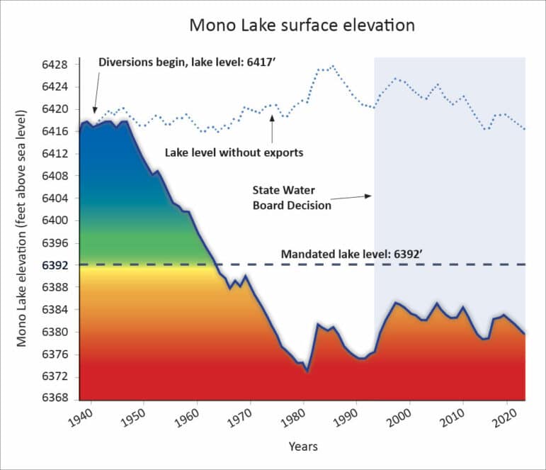
Mono Lake is part of the Owens Valley in the Eastern Sierra. Surface flow diversions and sustained groundwater pumping that started in 1905 in the Owens Valley provides up to 75% of the annual water supply for Los Angeles through the LA aqueduct. That water diversion has dropped the level of Mono Lake, increasing salinity and causing extreme dust storms (particulates - PM₁₀) from the exposed salts of the dried lakebed. Figure 12.2 shows the levels of Mono Lake over time and the timing of the State Water Board Decision to restore lake levels.

Figure 12.2: Mono Lake water elevation over time

12.2.1 Data

Lake levels
Historical water use along the LA aqueduct
Owens Valley PM₁₀ concentrations

12.3 Ecological Footprint and Biocapacity

The Global Footprint Network attempts to identify the ecological footprint of individuals and countries.

12.3.1 Definitions

12.3.1.1 Ecological Footprint

A measure of the area of biologically productive land and water required to (1) produce all the resources consumed by an individual, population, or activity and (2) absorb the waste generated. Units are in global hectares. A hectare is 100 acres or 10,000 m².

12.3.1.2 Biocapacity

A measure of the capacity of an ecosystem to regenerate biological resources. Biocapacity can change over time as a result of climate and management practices. It is calculated by multiplying area by yield factor and an equivalence factor and is measured in global hectares.

12.3.1.3 Global hectares

Global hectares are a measure of area weighted by the biological productive of the landtype. Global hectare is an earth averaged unit, but it may vary slightly over time because of changes in climate and management practices.

12.3.1.4 Ecological Deficit

The difference between the Biocapacity and Ecological Footprint of a region or country. When the footprint exceeds the biocapacity, a region or country runs an annual ecological deficit. Cumulative ecological deficits (and/or reserves) are the Ecological Footprint Networks measure of Ecological Debt.

12.3.2 Ecological Debt Case Study

The Footprint scenario tool is a measure of ecological debt in units of “Earth Debt”. Instead of comparing regions with local deficits or reserves, this tool estimates the cumulative ecological debt accumulated globally. It is a measure of the current unsustainable biological resource extraction and waste generation.

12.4 Los Angeles Water Supply

LA County runs an annual water deficit, which requires large annual imports of water from multiple sources. Let’s try to quantify these flows.

Let’s start with the supply of water data from the city of Los Angeles.

Here is a LADWP water supply in acre-feet.

library(janitor)


Attaching package: 'janitor'

The following objects are masked from 'package:stats':

    chisq.test, fisher.test

library(tidyverse)

── Attaching core tidyverse packages ──────────────────────── tidyverse 2.0.0 ──
✔ dplyr     1.1.2     ✔ readr     2.1.4
✔ forcats   1.0.0     ✔ stringr   1.5.0
✔ ggplot2   3.4.2     ✔ tibble    3.2.1
✔ lubridate 1.9.2     ✔ tidyr     1.3.0
✔ purrr     1.0.1

── Conflicts ────────────────────────────────────────── tidyverse_conflicts() ──
✖ dplyr::filter() masks stats::filter()
✖ dplyr::lag()    masks stats::lag()
ℹ Use the conflicted package (<http://conflicted.r-lib.org/>) to force all conflicts to become errors

H2O_data <- read_csv('https://data.lacity.org/api/views/qyvz-diiw/rows.csv?accessType=DOWNLOAD') %>% 
  clean_names()

Rows: 49 Columns: 11
── Column specification ────────────────────────────────────────────────────────
Delimiter: ","
chr (2): Date Value, Fiscal Year
dbl (9): MWD, LA Aqueduct, Local Groundwater, Recycled Water, Total Acre Fee...

ℹ Use `spec()` to retrieve the full column specification for this data.
ℹ Specify the column types or set `show_col_types = FALSE` to quiet this message.

12.4.0.1 Plot water supply over time

Figure 23.4 shows a simple bar chart of LA City water supply sources. Note that there is some fancy data manipulation first though. Also, there’s a call to the scales package to make the x-axis label nicer.

H2O_data %>% 
  select(1, 3:6) %>% 
  pivot_longer(names_to = 'parameter', values_to = 'acreFeet', cols = 2:5) %>% 
  mutate(date_value = lubridate::mdy_hms(date_value)) %>% 
  ggplot(aes(x = date_value, y = acreFeet, fill = parameter)) +
    #geom_line() +
    #geom_point() +
    geom_bar(stat = 'identity') +
    theme_bw() +
    scale_x_datetime(labels = scales::label_date_short(), date_breaks = '5 years') +
    labs(x = '', y = 'Supply in Acre Feet')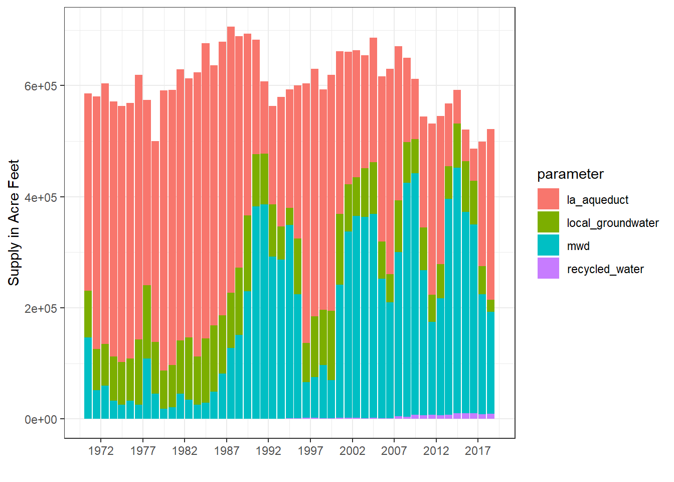

Figure 12.3: Water supply trends for LA City

12.4.1 Visualize Aqueducts in California

California Natural Resources Agency Open Data portal has an aqueduct layer.

Here’s the stepwise way to acquire and put this data for use. We’ll cover this in detail in the import lecture.

Download file - mine was named i12_Canals_and_Aqueducts_local.geojson
Move to working directory
Read file using read_sf()
Transform file to WGS84 using st_transform()
Make a map using leaflet() as shown in Figure 12.4 -
Refine map to only show aqueducts that serve LA County - a 5 minute attempt is shown here, getting it right may require research

library(sf)

Linking to GEOS 3.9.3, GDAL 3.5.2, PROJ 8.2.1; sf_use_s2() is TRUE

library(leaflet)
library(htmltools)

aqua <- read_sf(dsn = 'i12_Canals_and_Aqueducts_local.geojson') %>% 
   st_transform("+proj=longlat +ellps=WGS84 +datum=WGS84") 

#Team Debt needs to fill this in.
LACounty_aqua <- c('Main Canal', 'Los Angeles Aqueduct', 'Colorado River Aqueduct')

aqua %>% 
  filter(Name %in% LACounty_aqua) %>% 
  leaflet() %>% 
  addTiles() %>% 
  addPolylines(weight = 2,
              label = ~htmlEscape(Name))

Figure 12.4: Aqueducts providing water to LA county